Abstract
Most mainframe migration business cases get argued in MIPS, licenses and lines of code. The test that decides whether a migration survives its first month-end is simpler: does the nightly batch finish on time? This paper looks at what drives the elapsed time of sort steps on Linux, on premises or in the cloud. External sort is usually limited by the bytes the storage path can move, and processor speed matters less. Memory sets the number of passes over the data. And cloud storage puts layered, published ceilings on you that the mainframe’s channel subsystem never exposed. The paper treats the batch window as a critical-path problem, points out the traps that containers, record formats and network file systems bring in, and lays out a sizing method you can finish before cutover.
1. The batch window
IBM’s guidance on batch modernization says the batch window, “which can be different on different days of the week or month”, is set in the service-level agreement.1 The same Redbook says it’s not unusual to run 5,000 to 10,000 jobs in one evening, that job networks are different at weekends and month-end, and that the window keeps shrinking as online applications stay up longer, “sometimes up to 7x24”.1 Operators know it as batch that has to be done by a fixed hour.2
A migrated batch stream inherits those deadlines unchanged. It doesn’t inherit the machine that met them. Online services have to be back up at a stated time, downstream feeds have their own cut-offs, and month-end volumes run above the averages most sizing is based on. Sort sits between a lot of batch steps, so its elapsed time adds up along every chain of dependent jobs. On z/OS that elapsed time reflects an I/O subsystem that was sized once, for the whole shop, and it rarely shows up in a migration requirement. On Linux, and especially in the cloud, storage throughput is something you buy, with published limits. In this paper I’ll explain how the two connect. I’m not making claims here about any particular sort product.
2. How an external sort works
IBM describes a sort step as having three phases: input, work and output.2 When the data fits in the memory the sort has, the work phase is trivial. The data is read once and written once, and total storage traffic is twice the data volume. When it doesn’t fit, the sort reads the input in memory-sized pieces, sorts each piece and writes it to work files as a sorted run, then merges the runs into the output. Now the minimum is four transfers of the data: read the input, write the runs, read the runs, write the output.
Two things decide whether it needs more than that. The first is run length. A sort that fills memory, sorts and writes produces runs the size of memory. Replacement selection, the classic technique, produces runs that average about twice the size of memory on random input.3 The second is merge fan-in, the number of runs merged at once, which is limited by the buffer memory each input needs. GNU sort, the Linux utility, merges at most 16 inputs at once by default (its manual says the value is implementation-dependent) and writes intermediate files when there are more.4 When there are more runs than the fan-in, the sort does intermediate merges, and each one adds another read and write of the whole data volume. IBM’s Redpaper says “one of the most common tuning actions” for a sort step is to get rid of the work phase by getting rid of the intermediate merges.2
Where the CPU matters
A comparison sort does on the order of n log2 n comparisons, some 330 billion for ten billion records, and what each one costs depends on the key: how long it is, how many fields it spans, and whether they’re character, binary or packed decimal. For a fixed volume in bytes, short records mean more comparisons per gigabyte, and long records push the balance toward I/O. Reformatting, selection and summation, which mainframe control statements routinely combine with the sort, add more.
Compression trades CPU time for storage traffic. GNU sort can compress its temporary files through an external program.4 On z/OS, DFSORT cuts work data set I/O by using central storage, memory objects and hiperspaces where the system allows.7 Either one pays off when the sort is storage-bound and there’s spare CPU.
Exhibit 1. How memory and merge fan-in set a sort’s storage traffic (illustrative)
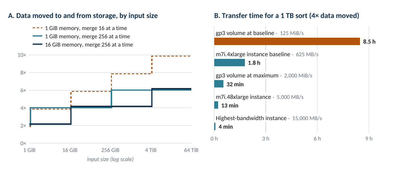
Panel A: modeled bytes read plus written, as a multiple of input size, assuming runs equal to memory and no compression. Lines are offset slightly where they coincide. Panel B: time to move 4 TB at each published ceiling, ignoring CPU and latency; ceilings from AWS documentation.5, 6 My own calculation. This isn’t a benchmark.
In Exhibit 1, with 16 GiB of memory and a wide merge, a sort of up to several terabytes needs one merge and moves four times its data. With 1 GiB and a fan-in of 16, a terabyte moves eight times its data. A 1 TB sort moving 4 TB through a path limited to 125 MiB/s spends about 8.5 hours just on transfers, which is longer than most batch windows. At 2,000 MiB/s it needs about half an hour.
3. Channels, volumes and instances
The mainframe keeps I/O separate from computation. System Assist Processors run the channel subsystem. An IBM z16 has between 5 and 24 standard SAPs depending on the model, and its channel subsystem architecture allows up to six channel subsystems of 256 channels each.8 FICON Express32S links on the z16 run at up to 32 Gbit/s.8 zHyperLink, IBM’s low-latency attachment, gives you an 8 GB/s link and up to ten times better response time than FICON for eligible operations. Only Db2 reads, Db2 log writes and VSAM data sets are eligible, over a point-to-point connection of at most 150 meters.9 The sequential data sets that sort reads and writes go over FICON. So what made a mainframe sort fast was aggregate channel and storage-controller bandwidth, shared by the whole shop and sized by its capacity planners.
In the cloud you buy that bandwidth in pieces, and each piece has a published ceiling (Exhibit 2). An AWS gp3 volume comes with 3,000 IOPS and 125 MiB/s, and since September 2025 you can provision it up to 80,000 IOPS and 2,000 MiB/s.5, 10 The instance adds a second limit. An m7i.large has a baseline EBS throughput of 81.25 MB/s and a maximum of 1,250 MB/s, and AWS says such instances “can sustain the maximum performance for 30 minutes at least once every 24 hours”.6 Google Cloud documents the same principle: a VM has its own IOPS and throughput limits across all the Hyperdisk volumes attached to it, and performance is capped by the lower of the disk and VM limits.11
Exhibit 2. Storage options and their published limits
| Option | Published ceiling | Note for sort |
|---|---|---|
| IBM z16 FICON Express32S | Up to 32 Gbit/s per link; up to 6 channel subsystems × 256 channels | Aggregate bandwidth sized per installation |
| IBM zHyperLink | 8 GB/s link; up to 10× better response time than FICON | Db2 and VSAM only; not sequential files |
| AWS EBS gp3 | Baseline 3,000 IOPS, 125 MiB/s; max 80,000 IOPS, 2,000 MiB/s | Baseline is what you get unless you provision more |
| AWS EBS io2 Block Express | Max 256,000 IOPS, 4,000 MiB/s | Provisioned-IOPS pricing |
| AWS EBS st1 (HDD) | 40 MiB/s per TiB baseline, 250 burst; 500 MiB/s max | Sequential I/O merged into 1 MiB units |
| AWS instance EBS limit | m7i.large 81.25 MB/s base (1,250 burst); m7i.4xlarge 625 base; m7i.48xlarge 5,000; highest listed 15,000 MB/s | Burst sustainable 30 min per 24 h |
| AWS instance store (NVMe) | i4i.32xlarge: 8 × 3,750 GB Nitro SSD | Lost on stop or terminate; work files only |
| Google Hyperdisk Balanced | Up to 160,000 IOPS, 2,400 MiB/s per volume | Also capped per VM |
| Google Hyperdisk Throughput | Up to 2,400 MiB/s per volume | HDD-like 10–30 ms read latency |
| Azure Premium SSD v2 | Baseline 3,000 IOPS, 125 MB/s; max 80,000 IOPS, 2,000 MB/s | VM limits also apply |
| Azure Ultra Disk | Max 400,000 IOPS, 10,000 MB/s | VM limits also apply |
| AWS EFS (NFS) | About 1 ms read, 2.7 ms write latency; 1,500 MiB/s per client | Latency on every operation; see Section 6 |
Sources: IBM Redbooks;8, 9 AWS, Google Cloud and Microsoft documentation as accessed September 2026.5, 6, 10–15 MiB/s = 220 bytes per second; MB/s = 106. Limits change, so check the current documentation before sizing.
That means three things for sort. First, the layers multiply. Striping four volumes gets you nothing if the instance limit is lower than their sum, and input, work and output files usually share the instance limit even when they’re on separate volumes. Second, I/O size matters. At 3,000 IOPS, a volume only reaches 125 MiB/s if the average request is about 43 KiB or bigger. A merge that uses small buffers to raise its fan-in issues smaller requests and can run out of IOPS before it runs out of bandwidth. Third, bursts mislead. A test run in the afternoon on a small instance may run entirely at burst rates, and a six-hour overnight stream won’t. HDD-class volumes like st1 build up and spend burst credits the same way.12
Local NVMe instance storage stays off the network and works well for sort work files, with one catch: its data is lost when the instance is stopped or terminated.13 Keep input and output on durable storage.
What the public benchmarks show
Sort has been a yardstick for computer systems since 1985, when an article in Datamation by Jim Gray and colleagues, published under the name Anon et al., proposed sorting a million 100-byte records as one of three standard measures.16 Gray founded the Sort Benchmark, which colleagues have kept going since he disappeared in 2007. Entries have to sort to and from operating-system files on secondary storage, using 100-byte records with random 10-byte keys.17
In 2014 a team from the University of California, San Diego sorted 100 TB with replication in 1,378 seconds in the Daytona GraySort category, and Databricks reported sorting 100 TB in 23 minutes on 206 machines with Apache Spark.18, 19 In 2016 a team from Nanjing University, Alibaba and Databricks set a CloudSort record of $1.44 per terabyte on 394 Alibaba Cloud nodes.19 The CloudSort record on sortbenchmark.org today is $0.97 per terabyte, set in 2022 by Exoshuffle-CloudSort on Amazon EC2 and S3.28 In 2019 KioxiaSort took the JouleSort record, sorting 1 TB in 8 minutes 45 seconds with 89 kJ of energy and a storage throughput of 7.6 GB/s.20
That last number tells you something. At 7.6 GB/s for 525 seconds, the system moved about 4 TB to sort 1 TB: four transfers of the data, exactly what the model in Section 2 predicts. Record-setting sorts are designed around storage bandwidth. As one research paper puts it, “the major bottleneck of external sorting is the latency associated with disk accesses”.21 Read the benchmarks as evidence of how the mechanism works. They aren’t sizing data. Their records are short, their keys random and single-field, and they do no reformatting. Commercial batch sorts are none of these things.
4. Running sorts in parallel
You can cut elapsed time by splitting the work: partitioning a big input by key range and sorting the partitions at the same time, or running independent sort steps side by side. Both only help while some resource is sitting idle. GNU sort defaults to one thread per available processor, limited to eight “as performance gains diminish after that”, with memory use going up by a factor of log n for n threads.4 Its manual also says an I/O-bound sort can often be sped up by putting temporary files on different file systems.4 Concurrent sorts on one instance share its throughput limit. If storage is the constraint, four sorts that each take an hour on their own won’t finish together in an hour.
Big servers add NUMA effects. The Linux kernel documentation explains that memory attached to the same cell as a processor is faster and has more bandwidth than memory on remote cells, and that tasks can migrate between nodes when things get out of balance.22 A multi-threaded sort with a large buffer is exactly the kind of workload that notices.
Containers and Kubernetes
More and more batch runs in containers, and their controls behave differently from z/OS workload management. On Linux, a CPU limit is enforced through CFS bandwidth control. A group gets a quota of CPU time in each period, and once the quota is used up its threads are throttled and “will not be able to run again until the next period”.23 Kubernetes describes a CPU limit as a hard limit the kernel enforces, and notes that containers aren’t terminated for using too much CPU.24 The step just takes longer. A sort with eight threads in a container limited to two CPUs spends a lot of each period throttled.
Memory is stricter. When a container uses more than its memory limit, “the kernel may terminate it”, and memory-backed tmpfs volumes count as container memory.24 A sort engine that sizes its buffer from the host’s physical memory, and ignores the container’s limit, can get killed at month-end volumes after running cleanly in test. Work files written to an ordinary emptyDir volume count as local ephemeral storage instead, and if a pod uses more than it’s allowed, the kubelet evicts it.25 Either way the step fails and starts over from the beginning, usually on the critical path.
5. Finding the critical path
A batch network is a set of jobs tied together by dependencies. It finishes when its longest chain of dependent jobs, the critical path, finishes. IBM’s Redpaper advises picking the jobs to tune from those on or near the critical paths,2 and the reason is arithmetic. Shortening a job that isn’t on the critical path doesn’t move the finish time at all. Shortening one that is moves it only until another chain becomes the longest.
Exhibit 3. A migrated nightly network that misses its window (hypothetical)
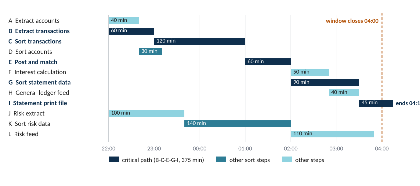
Hypothetical twelve-job network after migration, starting at 22:00, with each job at its earliest start. The durations are made up for illustration and don’t come from any installation.
In Exhibit 3 the window closes at 04:00, 360 minutes after the start. The critical path runs through the transaction extract, the transaction sort, posting, the statement sort and the print file, and ends at 04:15. Here are three fixes you might try.
- Halve the accounts sort (D). It has 110 minutes of slack. The network still ends at 04:15, so you save nothing.
- Cut the transaction sort (C) by 40 minutes. Its path drops to 335 minutes, but now the risk chain (J–K–L, 350 minutes) is critical. The network ends at 03:50. You were hoping to save 40 minutes and you saved 25.
- Cut C by 40 minutes and the risk sort (K) by 30. The network ends at 03:35, with 25 minutes to spare.
Whatever you gain by speeding up a step is capped by the gap to the next-longest path. The critical path at month-end or year-end often isn’t the one you see on an ordinary night, because the volumes and job networks are different,1 and a platform that’s slower on sort and faster elsewhere may meet the window or miss it depending entirely on which chain carries the sorts.
6. Two traps: record formats and network file systems
Mainframe sequential files are usually fixed-length (RECFM=FB) or variable-length (RECFM=VB). A variable record starts with a four-byte record descriptor word, and its first two bytes give the record length including the descriptor itself.26 File transfer tools used in text mode can strip or corrupt those descriptors. Line-sequential form, with a newline after each record, is only safe for character data. Packed-decimal and binary fields can contain the byte X’0A’, which Linux tools treat as the end of a line. Rehosting environments define their own conventions for variable-length files, and those aren’t necessarily byte-identical to a z/OS file with descriptors. Every change of format changes record lengths and key offsets, so settle the formats before you run any throughput test.
Network file systems are the second trap. They’re handy for passing files between jobs and between servers. They’re a poor place for sort work files, because every read and write of every pass goes across the network. AWS documents first-byte latencies for EFS of about 1 millisecond for reads and 2.7 milliseconds for writes, a per-client limit of 1,500 MiB/s in the best configuration and 500 MiB/s otherwise, and, in bursting mode, a baseline of 50 KiB/s per GiB stored. So a 1 TiB file system has a baseline of 50 MiB/s.15 A work directory left pointing at a shared mount, often because nobody changed a default, can turn a fast sort into a slow one. Keep shared file systems for handoffs.
7. How to size it
The evidence you need exists before the migration. Exhibit 4 turns it into a throughput requirement you can test. Fill it in for an ordinary night, for month-end and for year-end.
Exhibit 4. Batch window sizing checklist
| Step | What to find out | Evidence |
|---|---|---|
| 1. Map the window | Start time, hard deadlines, downstream cut-offs; ordinary night, month-end, year-end | SLAs; scheduler history |
| 2. Find the critical paths | Longest dependency chains and the slack on the next few | Scheduler plans; SMF type 30 step times |
| 3. Profile each sort on them | Bytes in and out, record format and length, key length and type, intermediate merges | SMF type 16; DFSORT messages |
| 4. Work out storage traffic | 2× data if it fits in memory, 4× for one merge, +2× per intermediate merge | Exhibit 1 model; memory budget |
| 5. Set throughput targets | Traffic ÷ time allowed on the critical path, for concurrent sorts together | Step 2 slack; concurrency plan |
| 6. Check every ceiling | Volume, instance and burst limits; IOPS at the planned I/O size | Provider documentation (Exhibit 2) |
| 7. Place the files | Work files on local NVMe or block storage; shared file systems only for handoffs | Mount and TMPDIR audit |
| 8. Set container limits | Memory limit above sort buffer plus overhead; ephemeral storage for work files; CPU limit versus threads | Pod specifications; throttling counters |
| 9. Test at peak volume | Full month-end data, overnight duration, past any burst allowance; agree a margin | Timed dress rehearsal |
SMF record types refer to the source z/OS system.27 Steps 2, 3 and 9 are the ones people skip most often.
Keep in mind that mainframe elapsed times already include that shop’s tuning, including DFSORT’s use of memory,7 so they aren’t a raw measure of the work.
8. Bottom line
- Size the storage path first. Once an external sort no longer fits in memory, it moves at least four times its data. Throughput per volume and per instance usually decides its elapsed time, much more than processor equivalence does.
- Buy memory before bandwidth. Getting rid of intermediate merges removes whole passes over the data, and IBM itself calls it one of the most common tuning actions.
- Read every ceiling, then rehearse. Cloud limits are published, but they stack, and some of them change over time. Container limits only fail at scale. Test at month-end volume for the full window.
- Work on the critical path. The longest chain of jobs decides whether you make the window. Improvements anywhere else cost money and change nothing.
References
1. IBM Redbooks, Batch Modernization on z/OS, SG24-7779-01, July 2012, §§1.3, 2.1, 2.3.3.
2. IBM Redbooks, Approaches to Optimize Batch Processing on z/OS, REDP-4816-00, October 2012, §§1.2, 2.2.5, 2.3.1.
3. D. E. Knuth, The Art of Computer Programming, Vol. 3: Sorting and Searching, 2nd ed., Addison-Wesley, 1998, §5.4.1.
4. GNU Coreutils manual, “sort invocation” (options --batch-size, --buffer-size, --compress-program, --parallel, -T), accessed September 2026.
5. AWS, Amazon EBS User Guide, “Amazon EBS volume types” and “Amazon EBS General Purpose SSD volumes”, accessed September 2026.
6. AWS, Amazon EC2 User Guide, “Amazon EBS-optimized instance types”, accessed September 2026.
7. IBM, z/OS DFSORT Tuning Guide (use of central storage, memory objects and Hipersorting).
8. IBM Redbooks, IBM z16 Technical Guide, SG24-8951.
9. IBM Redbooks, IBM zHyperLink for z/OS, REDP-5493, April 2022, updated May 2024.
10. AWS, “Amazon EBS increases the maximum size and provisioned performance of General Purpose (gp3) volumes”, 26 September 2025.
11. Google Cloud, Compute Engine documentation: “About Hyperdisk Balanced”, “About Hyperdisk Throughput”, “Hyperdisk performance overview”, accessed September 2026.
12. AWS, Amazon EBS User Guide, “Amazon EBS Throughput Optimized HDD and Cold HDD volumes”, accessed September 2026.
13. AWS, “Specifications for Amazon EC2 storage optimized instances” and Amazon EC2 I4i product page, accessed September 2026.
14. Microsoft, Azure Virtual Machines documentation, “Select a disk type for Azure IaaS VMs”, accessed September 2026.
15. AWS, Amazon EFS User Guide, “Amazon EFS performance specifications”, accessed September 2026.
16. Anon et al. [J. Gray and others], “A Measure of Transaction Processing Power”, Datamation, 1 April 1985.
17. ODBMS.org, “Sort Benchmark”, March 2014 (summary of benchmark rules and organizers).
18. M. Conley, University of California, San Diego, list of Sort Benchmark results, 2010–2014.
19. Databricks, press release on the CloudSort record, 15 November 2016 (also reporting the 2014 GraySort result).
20. Kioxia, “KioxiaSort set a world record in the sort benchmark contest”, 2019.
21. A. Kristo et al., “Parallel External Sorting of ASCII Records Using Learned Models”, arXiv:2305.05671, 2023.
22. Linux kernel documentation, “What is NUMA?”, Documentation/mm/numa.rst.
23. Linux kernel documentation, “CFS Bandwidth Control”, Documentation/scheduler/sched-bwc.rst.
24. Kubernetes documentation, “Resource Management for Pods and Containers”, accessed September 2026.
25. Kubernetes documentation, “Local ephemeral storage”, accessed September 2026.
26. IBM, z/OS DFSMS Using Data Sets (record formats and record descriptor words).
27. IBM, DFSORT SMF type 16 record and z/OS SMF type 30 record documentation.
28. Sort Benchmark, sortbenchmark.org, CloudSort results: NADSort (2016), Exoshuffle-CloudSort (2022), accessed September 2026.